Deployment Frequency
Definition and Purpose
Deployment Frequency (DF) traditionally measures how often a value stream successfully deploys a new version to production. It is one of the four key delivery performance metrics defined by the DevOps Research and Assessment (DORA). According to Accelerate1, high-performing organizations consistently deploy more frequently than low performers – not because they rush, but because their systems are designed for fast, reliable learning.
Deployment Frequency is therefore not primarily a speed metric. It is a learning metric that reflects how often the system can validate assumptions through real feedback.
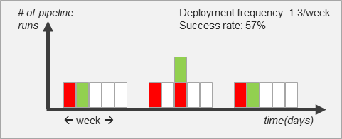
The graph shows pipeline activity over time, grouped into weekly blocks of five working days. Each vertical column represents one day.
- Green bars indicate a successful deployment (a completed hand-off to the next stage).
- Red bars represent a failed deployment attempt.
- White columns mean no deployment attempt was made on that day.
- Stacked bars indicate multiple pipeline runs on the same day; each bar has the same height and represents one run.
Deployment Frequency is calculated as the number of successful deployments (green bars) divided by the number of weeks shown.
In this example, the system achieves an average of 1.3 successful deployments per week.
Success Rate reflects pipeline reliability and is calculated as the ratio of successful runs to all attempted runs (green ÷ green + red).
Here, 57% of all pipeline runs were successful.
Together, Deployment Frequency and Success Rate show both how often the system delivers and how reliably it does so.
Deployment Frequency Beyond Production
In the context of large and complex value streams, the definition of Deployment Frequency is deliberately extended to include any successful hand-off from one stage to the next in the value stream – not just releases to production. Each stage in the value stream acts as a consumer of the previous one. Measuring Deployment Frequency at these hand-off points makes it possible to understand how often new versions are made available for integration, testing, or further development, long before a final release occurs.

Extending Deployment Frequency in this way moves it beyond a pure health and performance indicator and turns it into an analytical metric that reveals:
- where flow is constrained
- where feedback cycles are delayed or distorted
- where improvement efforts should start
Applied consistently across stages, Deployment Frequency highlights mismatches in cadence between components, subsystems, and integration levels, making systemic bottlenecks visible rather than hidden behind an aggregate system-level number.2
Why it Matters
Reliable product development depends not only on speed, but on fast and well-coordinated integration to enable early and meaningful feedback.
Many defects and design issues only surface once multiple components interact. The same is true for features that span modules, teams, or technical domains. If one component delivers infrequently or unreliably, downstream stages are forced to wait or work with outdated versions while new changes continue to arrive upstream. Work in progress increases3, and originally small changes begin to accumulate over time, merging into ever-larger effective batch sizes. As a result, feedback is delayed, integration effort grows, rework increases, and learning slows down across the entire system.
By measuring Deployment Frequency at each stage, organizations can identify which parts of the value stream limit learning and integration speed, even if the overall system appears healthy. This makes Deployment Frequency a key lever for improving end-to-end flow, reducing coordination friction, and accelerating feedback-driven development.
Where to Start Measuring Deployment Frequency
Deployment Frequency is best introduced incrementally. A practical starting point is the first stage where the system is fully integrated and assumptions about interactions, interfaces, and behavior are validated for the first time.
This initial integration point often represents the highest learning leverage in the value stream: many defects, design issues, and coordination problems only become visible once components interact in a realistic environment.
From there, Deployment Frequency can be extended upstream and downstream to build a stage-level view of learning cadence across the system. Other good starting points are stages that are particularly critical for overall flow, or stages where delays, quality issues, or coordination problems are already visible. Starting too broadly often hides local constraints; starting at these high-impact stages makes them visible and actionable.
Common Misinterpretations of Deployment Frequency
One of the most common misunderstandings is to treat Deployment Frequency primarily as a speed objective – assuming that delivering more often automatically means delivering better.
In practice, this often leads to the opposite effect. Systems begin to produce low-quality or unreliable outputs at a higher rate, increasing rework, instability, and coordination effort.4
A useful analogy is learning to play a difficult guitar solo. A skilled musician does not start by playing fast. They practice slowly and deliberately until timing, precision, and sound quality are correct. Only once the foundation is stable does increasing speed make sense. If a player tries to go faster before mastering the basics, the solo may become quicker – but it will sound rushed, imprecise, and awkward.
The equivalent foundation in a value stream is a clear Definition of Done and explicit acceptance criteria for deployment. A deployment should only be counted when these criteria are met – when the output is truly ready to be consumed by the next stage. Increasing Deployment Frequency without such standards in place merely accelerates the delivery of incomplete or unstable work.5
Deployment Frequency works the same way as practice speed. Sustainable gains emerge as a result of disciplined system improvement – stable pipelines, clear acceptance criteria, and reliable feedback – not as a shortcut to achieving it.
Deployment Frequency as a Leading Indicator
Deployment Frequency is a leading indicator. Changes in delivery cadence often become visible here before their impact shows up in lead time, quality metrics, or customer outcomes.
This makes Deployment Frequency particularly useful for validating whether structural improvements – such as automation, integration discipline, or architectural changes – are actually improving the system’s ability to learn.
Deployment Frequency in the Context of Other Flow and Quality Metrics
Deployment Frequency should never be interpreted in isolation. It describes how often a system creates opportunities for learning, but it does not indicate how effective that learning is.
High Deployment Frequency without a short Defect Resolution Time means that feedback is generated quickly but acted upon slowly. High Deployment Frequency combined with a high Defect Escape Rate means that learning occurs frequently, but too late to prevent downstream impact. In both cases, the system appears fast while remaining ineffective.
Only when Deployment Frequency improves together with fast defect resolution and early defect detection does increased delivery cadence translate into meaningful learning and sustained flow improvement.
References
- Forsgren, N., Humble, J., & Kim, G. (2018). Accelerate: The Science of Lean Software and DevOps. IT Revolution Press. ↩︎
- Deployment Frequency can be complemented by a release predictability metric that assesses the alignment between planned and delivered content over time. ↩︎
- Work in Progress (WIP) is captured by the Flow Load metric, which reflects how much work is currently active or waiting within the value stream. ↩︎
- After the initial publication of the DORA metrics, some organizations emphasized higher deployment counts without first establishing reliable pipelines and feedback mechanisms. Subsequent DORA research, as documented in Accelerate, clarified that sustainable performance requires both frequent and reliable delivery. ↩︎
- This implicitly assumes that each activity within the pipeline is continuously improved for reliability, resilience, and correctness. In the Assembly Line Model, this corresponds to the circles inside the blue boxes, which represent the individual activities that collectively determine the quality and stability of a stage’s output. ↩︎
Author: Peter Vollmer – Last Updated on Januar 15, 2026 by Peter Vollmer